Time complexity and Big-O notation

Shorter code is not necessarily faster, and a method that works well on small inputs may scale poorly. Time complexity compares how work grows as the input grows, rather than measuring one particular execution.

Time complexity

Time complexity describes the relationship between input size and the amount of work an algorithm performs. It helps compare algorithms independently of a specific machine or benchmark.

Big-O notation

Big-O describes an asymptotic upper bound on growth. Big-Omega gives a lower bound, and Big-Theta gives a tight bound. These are distinct from best-, average-, and worst-case inputs; an analysis can apply a bound to any of those cases. Worst-case Big-O is a common way to compare algorithms.

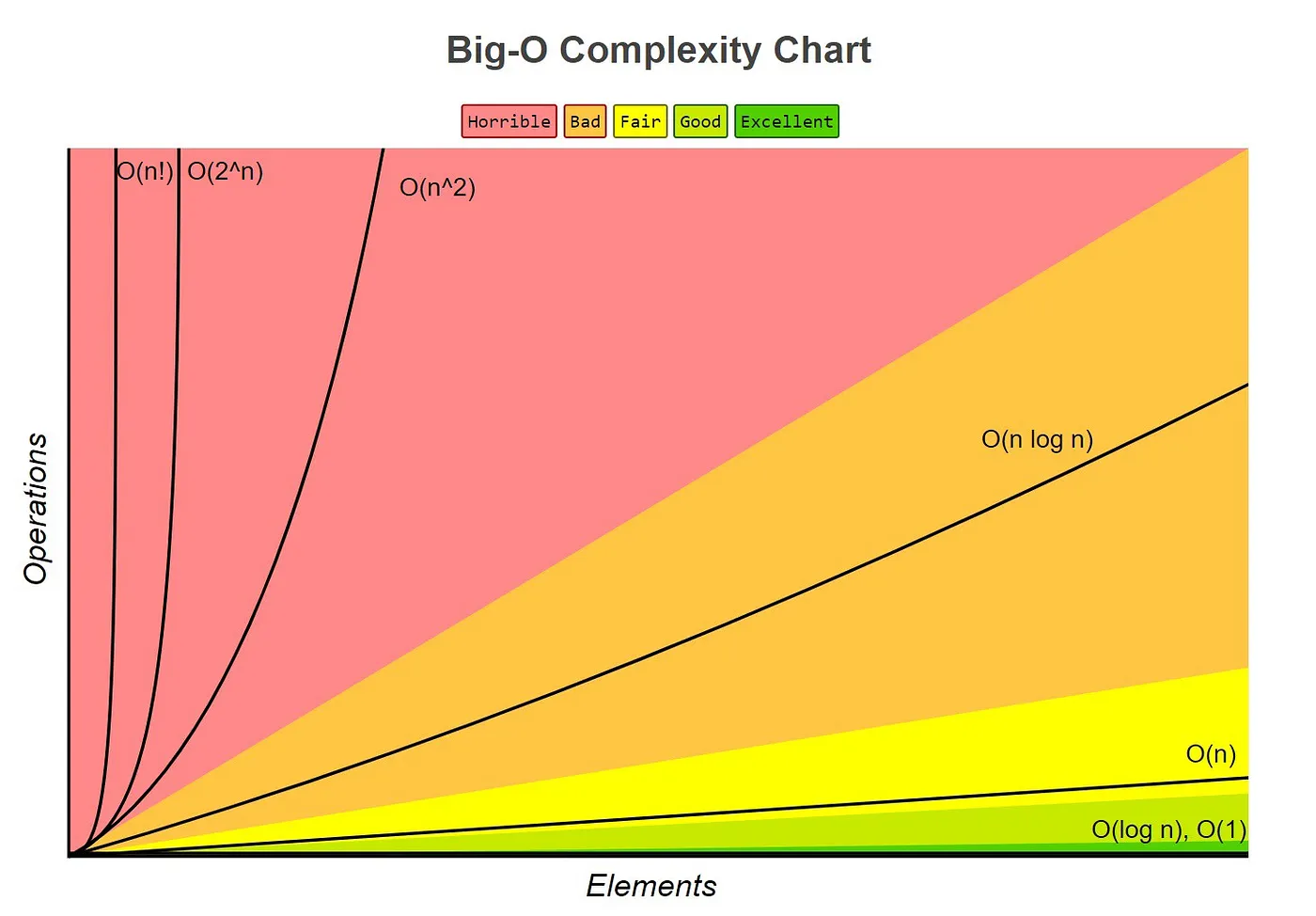
• Constant time: O(1)
  • The amount of work does not grow with the input size.
  • Example: accessing the first element of an array.
• Logarithmic time: O(log n)
  • Work grows slowly as each step reduces the remaining problem by a factor.
  • Example: binary search.
• Linear time: O(n)
  • Work grows in proportion to input size.
  • Example: visiting every element in a list.
• Linearithmic time: O(n log n)
  • Combines linear work with a logarithmic number of levels.
  • Examples: merge sort and quicksort on average.
• Quadratic time: O(n^2)
  • Work grows with the square of input size.
  • Example: nested loops that each traverse the input.
• Exponential time: O(2^n)
  • Work doubles with each additional input element.
  • Example: enumerating every subset of a set.

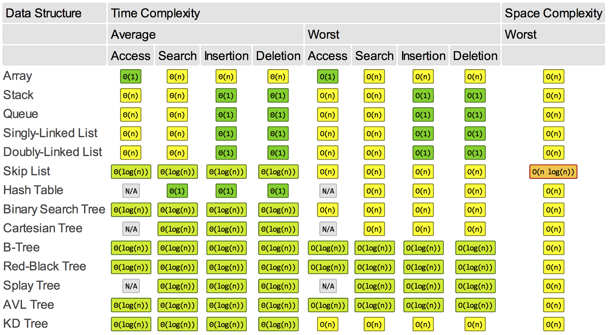
Data structures and complexity

Insertion, deletion, and lookup require different amounts of work depending on the data structure.

Further reading: MIT: Mathematics for Computer Science.